
Executive takeaway
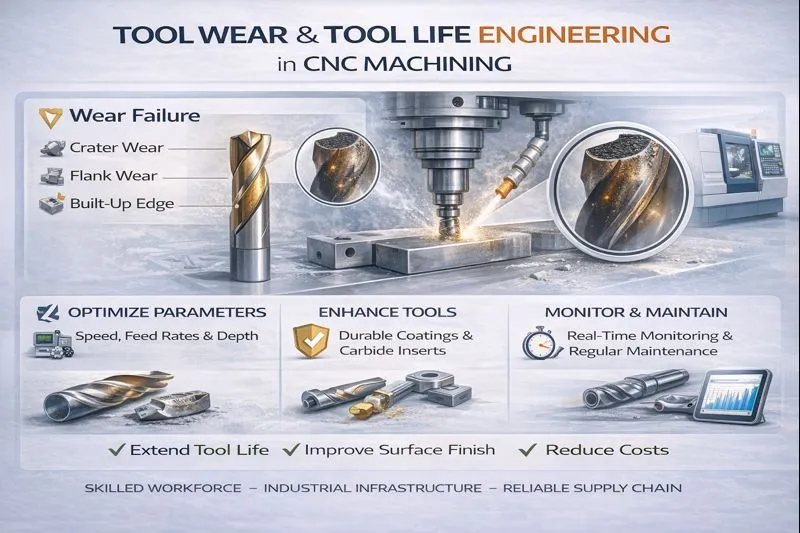
Tool wear is not a maintenance nuisance; it is a controlled process variable. In CNC machining, wear governs three outcomes buyers care about most: quality stability (dimension drift and surface integrity), delivery reliability (unplanned tool failures), and unit cost (cycle time versus tool-change frequency).
A mature machining system treats wear the same way it treats tolerances: it is defined, measured, modeled, and governed with clear decision rules. This article provides a practical, academically grounded approach built around four pillars:
- Mechanisms, not myths: distinguish what you see (wear pattern) from why it happens (wear mechanism).
- Defensible tool-life tests: design experiments that remain valid when audited or disputed (ISO 3685 mindset).
- Responsible models: use the Taylor tool-life equation as a local model inside a stable regime—not as a universal law.
- Production control: implement tool-change governance and tool-condition monitoring that improves robustness without flooding operators with false alarms.
1) First principles: what “tool wear” really is
1.1 Wear patterns vs wear mechanisms
Two vocabularies get mixed up in many factories:
- Wear patterns describe the geometry of damage you observe on the tool: flank wear, crater wear, notch wear, nose wear, edge chipping, thermal cracks.
- Wear mechanisms describe the physics and chemistry causing that pattern: abrasion, adhesion, diffusion/dissolution, oxidation/corrosion, thermal fatigue, mechanical fatigue, coating delamination.
Why the distinction matters: the same pattern can be produced by different mechanisms, and different mechanisms require different countermeasures. “Reduce speed” is not a universal fix; sometimes it makes things worse by pushing the cut into rubbing/ploughing regimes.
1.2 The wear curve (why wear accelerates late in life)
Most cutting tools follow a three‑stage wear progression:
- Break‑in (rapid micro‑geometry stabilization): edge rounding, coating polishing, small BUE events.
- Steady wear (approximately linear growth): flank land grows gradually; offset compensation is feasible.
- Accelerated wear (runaway): temperature rises, coatings fail locally, edge integrity degrades, and wear rate increases nonlinearly.
Production planning should aim to operate in Stage 2 and change tools before Stage 3. This is why “run to failure” is almost always the most expensive strategy.
1.3 A unifying wear model (Archard’s law as a mental model)
For many sliding‑wear systems, a useful conceptual model is Archard’s wear law:
Vw ≈ k · (W · s) / H
- Vw: worn volume
- k: wear coefficient (depends on tribology, temperature, coating, lubrication)
- W: normal load
- s: sliding distance
- H: hardness of the softer body (often the tool coating/substrate locally)
Metal cutting is more complex than pure sliding, but Archard’s law gives a disciplined intuition: wear increases with load, sliding distance, and the tribological coefficient that rises with heat and chemical interactions.
2) Wear patterns you see on the shop floor (and what they usually mean)
2.1 The main patterns
- Flank wear (VB): wear land on the clearance face. Usually gradual and predictable; often the basis of tool-life criteria.
- Crater wear (KT): wear on the rake face under chip flow. Strongly linked to temperature, diffusion, and chemical interactions.
- Notch wear: localized wear near the depth-of-cut line. Often tied to work‑hardened surfaces, oxidation, or interrupted contact conditions.
- Edge chipping / breakage: brittle fracture of the cutting edge, often due to vibration (chatter), impact, hard inclusions, or unstable engagement.
- Thermal cracking: repeated thermal cycling (especially with intermittent cuts or aggressive coolant application) produces crack networks.
- Built‑up edge (BUE): adhered work material forms and breaks off at the cutting edge, distorting geometry and roughness.
2.2 Pattern-to-action diagnostic table
The table below is not a “universal truth.” It is a starting diagnostic to organize hypotheses and choose quick experiments.
| Observed symptom | Likely dominant regime | Typical root causes | Fast production actions |
|---|---|---|---|
| Gradual flank wear; size drift is smooth | Stable, abrasive/adhesive wear | Normal wear; tool life near limit; chip-load OK | Set VB-based limit; add offset compensation schedule; verify coolant/filtration |
| Rapid crater wear; discoloration; surface integrity concerns | Thermal/diffusion dominated | Excessive temperature; poor coolant access; too high speed for tool/coating | Reduce speed or increase chip thickness; improve coolant delivery; change grade/coating |
| Notch wear at DOC line; sudden burr increase | Oxidation/work-hardened interaction | Hard scale/skin; interrupted contact; DOC aligned with hard layer | Change DOC; use lead-in strategy; different edge prep; consider pre-machining skin removal |
| Edge chipping; random failures; “perfect then suddenly bad” | Dynamic instability / impact | Chatter; interrupted cut; fixture compliance; hard inclusions | Reduce radial engagement; change toolpath to constant engagement; improve fixturing; change grade/toughness |
| High roughness spikes; BUE marks; unstable finish | Adhesion / rubbing regime | Too low chip thickness; dull edge; sticky material; improper coolant/lube | Increase chip thickness (feed per tooth); sharpen edge; use coating for adhesion control; adjust coolant/MQL |
| Thermal cracks; edge “crazing”; intermittent failures | Thermal fatigue | Severe thermal cycling; interrupted cut; aggressive coolant quenching hot edge | Stabilize thermal input; modify coolant strategy; change grade/coating; adjust entry/exit |
3) Wear mechanisms: the physics behind the patterns
3.1 Abrasion (hard particles / hard phases)
Abrasion is driven by hard asperities or inclusions ploughing the tool surface. It is common when machining materials with hard phases (carbides, oxides) or when recut chips are present. Abrasion tends to produce steady flank wear and can be mitigated by coatings with high hardness and by improving chip evacuation.
3.2 Adhesion (micro-welding and tearing)
Adhesion occurs when workpiece material bonds to the tool at high local pressure and temperature, then tears away tool material or changes edge geometry. Adhesion is closely linked to BUE. It is sensitive to chip thickness (rubbing vs cutting), tool edge prep, and lubrication chemistry.
3.3 Diffusion / dissolution (high-temperature chemical wear)
At elevated temperatures, atoms can diffuse between tool and chip, weakening the tool and accelerating crater wear. This mechanism is strongly influenced by tool material, coating, and temperature at the tool-chip interface. The operational translation is simple: if crater wear accelerates, your process is running too hot for the tool system.
3.4 Oxidation and corrosion wear
Oxidation can form brittle layers that spall, particularly at the depth-of-cut line where oxygen access and temperature gradients differ. This is one reason notch wear often appears at the DOC boundary. Coolant chemistry, cutting environment, and temperature control matter.
3.5 Mechanical fatigue and thermal fatigue
In interrupted cuts, the cutting edge experiences cyclic mechanical loading and cyclic heating/cooling. Micro-cracks can initiate and propagate, leading to chipping or catastrophic breakage. Tool toughness, edge prep, and stable engagement strategies become decisive.
3.6 The “wear map” mindset
Rather than chasing single variables, treat wear as a regime map across:
- temperature (increasing with cutting speed, poor coolant access, rubbing)
- contact pressure (increasing with chip thickness, negative rake, hard materials)
- sliding distance (related to cutting length and chip flow)
- chemistry (coating, coolant/lube, work material)
Most “mystery wear” is a regime change: a small change in engagement, coolant delivery, or chip formation moves the system into a different dominant mechanism.
4) Tool life: definitions and defensible testing (ISO 3685 mindset)
4.1 What “tool life” is (and what it is not)
Tool life is the cutting time (or cutting length / number of parts) until a defined end‑of‑life criterion is reached. The criterion must be stated. Common criteria include:
- Flank wear land reaching a specified value (VB or VBmax)
- Crater wear reaching a specified depth (KT)
- Surface roughness or dimensional drift exceeding a CTQ limit
- Catastrophic failure (edge fracture) — generally undesirable as a planned criterion
ISO 3685 provides recommended procedures for tool‑life testing with single‑point turning tools, including factors like workpiece, tool, cutting fluid, cutting conditions, and how to record and present results. Using a standards mindset makes your results comparable, repeatable, and credible.
4.2 A production-grade tool-life experiment design
A tool-life test that produces useful, transferrable constants must control the variables that actually move wear regimes. A robust design includes:
- Workpiece definition: alloy, condition, hardness range, and a plan for lot variability.
- Tool system definition: grade, coating, edge prep, nose radius, toolholder/runout control.
- Cut definition: speed, feed, depth of cut, engagement strategy, coolant strategy.
- Wear measurement protocol: how, where, and how often you measure VB/KT; magnification and repeatability.
- Stop rules: a clearly defined wear limit or quality limit; do not “run to failure” unless the purpose is failure-mode characterization.
4.3 Measurement discipline: wear measurement is an MSA problem
Wear measurement can be noisy: lighting, microscope focus, operator judgment, and tool cleaning can change readings. If you do not control measurement variation, you will fit the noise instead of the physics. Treat wear measurement like metrology:
- Standardize tool cleaning and imaging conditions.
- Use the same reference location on the edge for VB measurements.
- Record uncertainty qualitatively at minimum; quantify if tool-life constants will be used contractually.
5) Modeling tool life: Taylor equation, extensions, and honest boundaries
5.1 The Taylor tool-life equation (local model)
A widely used empirical relationship between cutting speed V and tool life T is the Taylor equation:
V · Tn = C
Where n and C are constants determined experimentally for a specific tool–work material system under a defined set of conditions. This relationship is foundational in metal cutting education and remains useful in production when applied correctly.
5.2 How to fit n and C correctly (log-linear regression)
Taking logs:
log V = log C − n · log T
So the slope of log V vs log T is −n. In practice:
- Run controlled tests at 3–6 cutting speeds (and ideally replicate at least one point).
- Measure tool life by a stated criterion (e.g., VB limit).
- Fit a line in log space; check residuals (regime changes show up as curvature or outliers).
5.3 Quick estimation from two points (useful for pilots, not for contracts)
If you only have two test points (V1, T1) and (V2, T2):
n = (log V1 − log V2) / (log T2 − log T1)
Then C = V · Tn for either point. This is sensitive to measurement noise and should be treated as provisional.
5.4 Generalized Taylor equation (when feed and depth matter)
A more general empirical form includes feed and depth of cut:
V · Tn · fa · db = C
Use this only if you have enough data to identify the exponents and if your process truly varies those parameters across production. Otherwise, you will overfit and create a fragile model.
5.5 The boundary rule: Taylor constants are not portable across regime changes
The Taylor equation is most reliable inside a stable regime—same tool grade/coating, similar chip formation mode, similar coolant access, and similar engagement strategy. If you change any of the following, expect constants to change:
- tool grade/coating or edge prep
- coolant strategy (flood vs MQL vs dry) or coolant access
- engagement strategy (slotting vs adaptive/constant engagement)
- material condition (hardness, microstructure, work-hardening behavior)
6) Turning wear into quality risk: how wear creates defects
6.1 Dimensional drift model (the offset-compensable zone)
In many operations, early flank wear causes a gradual effective radius change. If the tool geometry remains stable (no chipping), you can often compensate with offsets. The key is to define an offset-compensable wear window and a hard stop before edge integrity collapses.
6.2 When offsets cannot save you
Offsets do not fix geometry when wear changes the effective cutting edge shape in a non-repeatable way:
- edge chipping changes local edge geometry randomly
- notch wear changes the effective depth-of-cut boundary and can drive burrs
- thermal cracking produces sudden failure risk
- BUE creates stochastic geometry and surface defects
These are regime problems, not offset problems.
6.3 Surface integrity and wear: beyond Ra
As wear increases, cutting temperature and rubbing can rise, affecting near-surface microstructure, residual stress, and surface damage. Even if roughness (Ra) remains acceptable, functional performance can degrade (fatigue, sealing stability, friction). This is why high-reliability machining systems treat wear as a surface-integrity variable, not just a dimensional one.
7) Economical tool life: optimizing speed is a cost model problem
The “best” cutting speed is rarely the one that maximizes tool life. Production optimization balances machine time versus tool change cost. A simple model:
- Cm: machine cost per minute (including overhead)
- t: machining time per part (depends on speed)
- Ct: tool cost per change (insert + labor + lost time)
- T: tool life in minutes
Approximate tool cost per part as Ct · (t / T). Total cost per part becomes:
Cpart ≈ Cm · t + Ct · (t / T)
Because T decreases with speed via the Taylor equation, the optimal speed is a compromise. The practical implication: if you reduce speed slightly, tool life can increase disproportionately (depending on n), and total cost may drop if tool changes are expensive or risk is high.
8) Tool condition monitoring (TCM): from theory to production without false alarms
8.1 Direct vs indirect monitoring
- Direct: measure wear by imaging the tool (requires interruption).
- Indirect: infer wear from sensors around the process (power/current, vibration, acoustic emission, force proxies, temperature).
Indirect tool condition monitoring has a rich literature and can be production-viable when designed around stable features and clear decision rules.
8.2 Signal pipeline (the part most systems get wrong)
A robust monitoring system has five layers:
- Define the unit of monitoring: per tool? per operation? per NC segment? Choose the level that is repeatable.
- Acquire signals: power/current, vibration, AE, forces; sample rate appropriate to phenomenon.
- Pre-process: remove transients (entry/exit), normalize for feed/speed, filter noise.
- Extract features: RMS power, spectral peaks, kurtosis, envelope features, force coefficients.
- Decide: thresholds + trend rules + confirmation logic to avoid false alarms.
8.3 The “three failure modes” of TCM in real factories
- False alarms (operators ignore it): caused by poor normalization, program transients, or material variation.
- Missed detection (catastrophic breakage still happens): caused by too-slow sampling, too-high thresholds, or monitoring the wrong operation segment.
- Non-transferability (works on one machine, fails on another): caused by sensor placement differences, spindle dynamics differences, or inconsistent baselines.
8.4 A pragmatic high-mix strategy
High-mix machining makes monitoring harder because “normal” varies. A practical approach is to:
- Define signature windows in the program (stable engagement segments) and monitor only those.
- Store a baseline signature for each tool-operation-material family.
- Use trend-based rules (rate of change) rather than absolute thresholds when possible.
- Combine monitoring with conservative tool-change limits until confidence is proven.
9) Production control plan template (what “tool wear control” looks like)
9.1 Qualification stage
- Run a tool-life qualification (ISO 3685 mindset) for each critical operation family.
- Define end-of-life criteria: VB/KT limits and/or CTQ drift limits.
- Define tool-change interval with safety margin (avoid accelerated wear zone).
9.2 Routine production stage
- Tool governance: controlled tool library, grade/coating revision control, insert batch traceability when warranted.
- Offset policy: when offsets are allowed, how often, and by how much; who approves changes.
- Monitoring policy: which operations are monitored, which signals, what thresholds, and what reaction plan.
- Verification policy: sampling plan for CTQs sensitive to wear; escalation triggers.
9.3 Reaction plan (the most important page)
Every shop has a “tool wear policy.” Very few have a reaction plan that prevents repeated escapes. Your reaction plan should define:
- What happens when wear reaches limit early (stop, quarantine, root cause, retest).
- What happens when monitoring triggers an alarm (confirm, change tool, inspect last N parts).
- How to handle suspected regime change (coolant issue, material issue, fixture issue).
10) Buyer-grade evidence (industry-agnostic)
If you want to convince demanding customers, present evidence that is reproducible and auditable:
- Tool-life qualification summary: conditions, criterion, results, and safety margin.
- Control plan excerpt: tool-change limits, offset rules, inspection plan for wear-sensitive CTQs.
- Process stability data: CTQ trends across tool life (first part to last part).
- Change control: what triggers re-qualification (tool grade change, coolant strategy change, new material source).
FAQ (production intent)
- Is it better to maximize tool life or to maximize productivity?
Neither in isolation. Optimize total cost and delivery risk by balancing cycle time with tool-change frequency and scrap risk. - Why did the tool suddenly start chipping when it was fine yesterday?
Sudden chipping usually indicates a regime change: chatter, harder material zone, interrupted engagement, coolant loss, or edge fatigue reaching a threshold. - Can offsets compensate for tool wear?
Only while wear is gradual and geometry remains stable. Offsets cannot correct random chipping, notch wear effects, or BUE-driven surface defects. - Do I need ISO 3685 testing for milling?
ISO 3685 is for single-point turning, but the mindset—controlled variables, stated criteria, defensible reporting—applies to milling tool-life qualification as well. - What is the simplest TCM signal to start with?
Spindle power/current is often the most accessible. Start with stable operation segments and trend-based thresholds.
Conclusion
Tool wear becomes manageable when you stop treating it as unpredictable. Build a system that (1) understands mechanisms, (2) qualifies tool life with controlled tests, (3) uses models inside valid regimes, and (4) governs production with clear tool-change rules and monitoring that operators trust. This is how machining organizations protect quality, lead time, and unit cost—at scale.